Visualizing Solvers with TensorBoard
This tutorial may assume knowledge from the tutorial on Visualization with TensorBoard. It is based on MinPy’s CNN Tutorial.
Equip the CNN Tutorial with Visualization Functions
Set up as in the original tutorial.
In [1]:
"""Convolution Neural Network example using only MXNet symbol."""
import sys

from minpy.nn.io import NDArrayIter
# Can also use MXNet IO here
# from mxnet.io import NDArrayIter
from minpy.core import Function
from minpy.nn import layers
from minpy.nn.model import ModelBase
from minpy.nn.solver import Solver
from examples.utils.data_utils import get_CIFAR10_data

# Please uncomment following if you have GPU-enabled MXNet installed.
#from minpy.context import set_context, gpu
#set_context(gpu(0)) # set the global context as gpu(0)

import mxnet as mx

batch_size=128
input_size=(3, 32, 32)
flattened_input_size=3 * 32 * 32
hidden_size=512
num_classes=10
Design a template for CNN.
In [2]:
class ConvolutionNet(ModelBase):
    def __init__(self):
        super(ConvolutionNet, self).__init__()
        # Define symbols that using convolution and max pooling to extract better features
        # from input image.
        net = mx.sym.Variable(name='X')
        net = mx.sym.Convolution(
                data=net, name='conv', kernel=(7, 7), num_filter=32)
        net = mx.sym.Activation(
                data=net, act_type='relu')
        net = mx.sym.Pooling(
                data=net, name='pool', pool_type='max', kernel=(2, 2),
                stride=(2, 2))
        net = mx.sym.Flatten(data=net)
        net = mx.sym.FullyConnected(
                data=net, name='fc1', num_hidden=hidden_size)
        net = mx.sym.Activation(
                data=net, act_type='relu')
        net = mx.sym.FullyConnected(
                data=net, name='fc2', num_hidden=num_classes)
        net = mx.sym.SoftmaxOutput(data=net, name='softmax', normalization='batch')
        # Create forward function and add parameters to this model.
        input_shapes = {'X': (batch_size,) + input_size, 'softmax_label': (batch_size,)}
        self.cnn = Function(net, input_shapes=input_shapes, name='cnn')
        self.add_params(self.cnn.get_params())

    def forward_batch(self, batch, mode):
        out = self.cnn(X=batch.data[0],
                       softmax_label=batch.label[0],
                       **self.params)
        return out

    def loss(self, predict, y):
        return layers.softmax_cross_entropy(predict, y)
Set get_CIFAR10_data’s argument to the data file location for
cifar-10 dataset. The original tutorial applied an argparse to read the
directory directly in the terminal. For the convenience of using a
Jupyter notebook, this is not used here.
Declare the directory for storing log files, which will be used for viusalization later.
visualize is an optional argument of Solver and is set to be
False by default. Set visualize to be True and pass the
summaries_dir argument as well. We will touch the details of
implementing visualization functions in Solver later.
In [3]:
def main():
    # Create model.
    model = ConvolutionNet()
    # Create data iterators for training and testing sets.
    data = get_CIFAR10_data('cifar-10-batches-py')
    train_dataiter = NDArrayIter(data=data['X_train'],
                                 label=data['y_train'],
                                 batch_size=batch_size,
                                 shuffle=True)
    test_dataiter = NDArrayIter(data=data['X_test'],
                                label=data['y_test'],
                                batch_size=batch_size,
                                shuffle=False)

    # Declare the directory for storing data, which will be used for visualization with tensorboard later.
    summaries_dir = '/private/tmp/cnn_log'

    # Create solver.
    solver = Solver(model,
                    train_dataiter,
                    test_dataiter,
                    num_epochs=10,
                    init_rule='gaussian',
                    init_config={
                        'stdvar': 0.001
                    },
                    update_rule='sgd_momentum',
                    optim_config={
                        'learning_rate': 1e-3,
                        'momentum': 0.9
                    },
                    verbose=True,
                    print_every=20,
                    visualize=True,
                    summaries_dir=summaries_dir)
    # Initialize model parameters.
    solver.init()
    # Train!
    solver.train()
In [4]:
if __name__ == '__main__':
    main()
(Iteration 1 / 3828) loss: 2.302535
(Iteration 21 / 3828) loss: 2.302051
(Iteration 41 / 3828) loss: 2.291640
(Iteration 61 / 3828) loss: 2.133044
(Iteration 81 / 3828) loss: 2.033680
(Iteration 101 / 3828) loss: 1.995795
(Iteration 121 / 3828) loss: 1.796180
(Iteration 141 / 3828) loss: 1.884282
(Iteration 161 / 3828) loss: 1.702727
(Iteration 181 / 3828) loss: 1.745341
(Iteration 201 / 3828) loss: 1.550407
(Iteration 221 / 3828) loss: 1.405793
(Iteration 241 / 3828) loss: 1.529175
(Iteration 261 / 3828) loss: 1.440347
(Iteration 281 / 3828) loss: 1.859766
(Iteration 301 / 3828) loss: 1.416149
(Iteration 321 / 3828) loss: 1.481019
(Iteration 341 / 3828) loss: 1.501948
(Iteration 361 / 3828) loss: 1.508027
(Iteration 381 / 3828) loss: 1.516997
(Epoch 1 / 10) train acc: 0.501953125, val_acc: 0.4931640625, time: 1253.37731194.
(Iteration 401 / 3828) loss: 1.296929
(Iteration 421 / 3828) loss: 1.496588
(Iteration 441 / 3828) loss: 1.330925
(Iteration 461 / 3828) loss: 1.450040
(Iteration 481 / 3828) loss: 1.393043
(Iteration 501 / 3828) loss: 1.239604
(Iteration 521 / 3828) loss: 1.210205
(Iteration 541 / 3828) loss: 1.295574
(Iteration 561 / 3828) loss: 1.372109
(Iteration 581 / 3828) loss: 1.231615
(Iteration 601 / 3828) loss: 1.243544
(Iteration 621 / 3828) loss: 1.313342
(Iteration 641 / 3828) loss: 1.510346
(Iteration 661 / 3828) loss: 1.155001
(Iteration 681 / 3828) loss: 1.241223
(Iteration 701 / 3828) loss: 1.305725
(Iteration 721 / 3828) loss: 1.218895
(Iteration 741 / 3828) loss: 1.208463
(Iteration 761 / 3828) loss: 1.319934
(Epoch 2 / 10) train acc: 0.5751953125, val_acc: 0.5517578125, time: 1238.14002705.
(Iteration 781 / 3828) loss: 1.204560
(Iteration 801 / 3828) loss: 1.388396
(Iteration 821 / 3828) loss: 1.208335
(Iteration 841 / 3828) loss: 1.197055
(Iteration 861 / 3828) loss: 1.225983
(Iteration 881 / 3828) loss: 1.007661
(Iteration 901 / 3828) loss: 1.083537
(Iteration 921 / 3828) loss: 1.170273
(Iteration 941 / 3828) loss: 1.079046
(Iteration 961 / 3828) loss: 1.060466
(Iteration 981 / 3828) loss: 1.186217
(Iteration 1001 / 3828) loss: 1.176932
(Iteration 1021 / 3828) loss: 1.049240
(Iteration 1041 / 3828) loss: 1.084303
(Iteration 1061 / 3828) loss: 1.137581
(Iteration 1081 / 3828) loss: 1.201812
(Iteration 1101 / 3828) loss: 0.991179
(Iteration 1121 / 3828) loss: 1.053682
(Iteration 1141 / 3828) loss: 1.033876
(Epoch 3 / 10) train acc: 0.5771484375, val_acc: 0.5859375, time: 1111.29330206.
(Iteration 1161 / 3828) loss: 0.945752
(Iteration 1181 / 3828) loss: 0.900214
(Iteration 1201 / 3828) loss: 0.996316
(Iteration 1221 / 3828) loss: 0.725004
(Iteration 1241 / 3828) loss: 1.053474
(Iteration 1261 / 3828) loss: 0.956877
(Iteration 1281 / 3828) loss: 1.118823
(Iteration 1301 / 3828) loss: 1.032918
(Iteration 1321 / 3828) loss: 1.078873
(Iteration 1341 / 3828) loss: 0.964023
(Iteration 1361 / 3828) loss: 1.081211
(Iteration 1381 / 3828) loss: 0.975109
(Iteration 1401 / 3828) loss: 0.887941
(Iteration 1421 / 3828) loss: 0.812622
(Iteration 1441 / 3828) loss: 0.781776
(Iteration 1461 / 3828) loss: 0.839401
(Iteration 1481 / 3828) loss: 1.083514
(Iteration 1501 / 3828) loss: 0.916411
(Iteration 1521 / 3828) loss: 0.820561
(Epoch 4 / 10) train acc: 0.658203125, val_acc: 0.599609375, time: 1107.30718303.
(Iteration 1541 / 3828) loss: 0.956412
(Iteration 1561 / 3828) loss: 0.835572
(Iteration 1581 / 3828) loss: 0.791931
(Iteration 1601 / 3828) loss: 0.892034
(Iteration 1621 / 3828) loss: 0.846968
(Iteration 1641 / 3828) loss: 0.790181
(Iteration 1661 / 3828) loss: 1.008565
(Iteration 1681 / 3828) loss: 0.971547
(Iteration 1701 / 3828) loss: 0.904101
(Iteration 1721 / 3828) loss: 0.764249
(Iteration 1741 / 3828) loss: 0.839634
(Iteration 1761 / 3828) loss: 0.667381
(Iteration 1781 / 3828) loss: 0.892126
(Iteration 1801 / 3828) loss: 0.790432
(Iteration 1821 / 3828) loss: 0.915785
(Iteration 1841 / 3828) loss: 0.701808
(Iteration 1861 / 3828) loss: 0.713519
(Iteration 1881 / 3828) loss: 0.939402
(Iteration 1901 / 3828) loss: 0.728612
(Epoch 5 / 10) train acc: 0.6630859375, val_acc: 0.5966796875, time: 1127.98228502.
(Iteration 1921 / 3828) loss: 0.898663
(Iteration 1941 / 3828) loss: 1.081481
(Iteration 1961 / 3828) loss: 0.956133
(Iteration 1981 / 3828) loss: 0.664632
(Iteration 2001 / 3828) loss: 0.986162
(Iteration 2021 / 3828) loss: 0.921607
(Iteration 2041 / 3828) loss: 0.855872
(Iteration 2061 / 3828) loss: 0.785384
(Iteration 2081 / 3828) loss: 0.985731
(Iteration 2101 / 3828) loss: 0.693248
(Iteration 2121 / 3828) loss: 1.032196
(Iteration 2141 / 3828) loss: 0.918029
(Iteration 2161 / 3828) loss: 0.809714
(Iteration 2181 / 3828) loss: 0.876201
(Iteration 2201 / 3828) loss: 0.714913
(Iteration 2221 / 3828) loss: 0.964526
(Iteration 2241 / 3828) loss: 0.795892
(Iteration 2261 / 3828) loss: 0.756644
(Iteration 2281 / 3828) loss: 0.571955
(Epoch 6 / 10) train acc: 0.720703125, val_acc: 0.6044921875, time: 1100.48066902.
(Iteration 2301 / 3828) loss: 0.584125
(Iteration 2321 / 3828) loss: 0.818221
(Iteration 2341 / 3828) loss: 0.647816
(Iteration 2361 / 3828) loss: 0.807244
(Iteration 2381 / 3828) loss: 0.663801
(Iteration 2401 / 3828) loss: 0.710950
(Iteration 2421 / 3828) loss: 0.869763
(Iteration 2441 / 3828) loss: 0.659388
(Iteration 2461 / 3828) loss: 0.884262
(Iteration 2481 / 3828) loss: 0.892994
(Iteration 2501 / 3828) loss: 0.696201
(Iteration 2521 / 3828) loss: 0.792361
(Iteration 2541 / 3828) loss: 0.583030
(Iteration 2561 / 3828) loss: 0.987736
(Iteration 2581 / 3828) loss: 0.812939
(Iteration 2601 / 3828) loss: 0.686343
(Iteration 2621 / 3828) loss: 0.696793
(Iteration 2641 / 3828) loss: 0.730227
(Iteration 2661 / 3828) loss: 0.717481
(Iteration 2681 / 3828) loss: 0.717061
(Epoch 7 / 10) train acc: 0.6875, val_acc: 0.5849609375, time: 1019.18220496.
(Iteration 2701 / 3828) loss: 0.960259
(Iteration 2721 / 3828) loss: 0.851661
(Iteration 2741 / 3828) loss: 0.547349
(Iteration 2761 / 3828) loss: 0.629300
(Iteration 2781 / 3828) loss: 0.794492
(Iteration 2801 / 3828) loss: 0.674677
(Iteration 2821 / 3828) loss: 0.547635
(Iteration 2841 / 3828) loss: 0.633213
(Iteration 2861 / 3828) loss: 0.817622
(Iteration 2881 / 3828) loss: 0.759713
(Iteration 2901 / 3828) loss: 0.746527
(Iteration 2921 / 3828) loss: 0.809928
(Iteration 2941 / 3828) loss: 0.804247
(Iteration 2961 / 3828) loss: 0.593531
(Iteration 2981 / 3828) loss: 0.884193
(Iteration 3001 / 3828) loss: 0.645554
(Iteration 3021 / 3828) loss: 0.568051
(Iteration 3041 / 3828) loss: 0.523802
(Iteration 3061 / 3828) loss: 0.691015
(Epoch 8 / 10) train acc: 0.6953125, val_acc: 0.5947265625, time: 962.428817034.
(Iteration 3081 / 3828) loss: 0.646333
(Iteration 3101 / 3828) loss: 0.893681
(Iteration 3121 / 3828) loss: 0.822102
(Iteration 3141 / 3828) loss: 0.619557
(Iteration 3161 / 3828) loss: 0.787171
(Iteration 3181 / 3828) loss: 0.725924
(Iteration 3201 / 3828) loss: 0.559321
(Iteration 3221 / 3828) loss: 0.654796
(Iteration 3241 / 3828) loss: 0.646047
(Iteration 3261 / 3828) loss: 0.789430
(Iteration 3281 / 3828) loss: 0.639559
(Iteration 3301 / 3828) loss: 0.798087
(Iteration 3321 / 3828) loss: 0.669927
(Iteration 3341 / 3828) loss: 0.706900
(Iteration 3361 / 3828) loss: 0.560583
(Iteration 3381 / 3828) loss: 0.630658
(Iteration 3401 / 3828) loss: 0.804180
(Iteration 3421 / 3828) loss: 0.727579
(Iteration 3441 / 3828) loss: 0.547852
(Epoch 9 / 10) train acc: 0.6982421875, val_acc: 0.5888671875, time: 958.027697086.
(Iteration 3461 / 3828) loss: 0.599252
(Iteration 3481 / 3828) loss: 0.485362
(Iteration 3501 / 3828) loss: 0.741121
(Iteration 3521 / 3828) loss: 0.636478
(Iteration 3541 / 3828) loss: 0.711437
(Iteration 3561 / 3828) loss: 0.655215
(Iteration 3581 / 3828) loss: 0.651631
(Iteration 3601 / 3828) loss: 0.762882
(Iteration 3621 / 3828) loss: 0.817763
(Iteration 3641 / 3828) loss: 0.768698
(Iteration 3661 / 3828) loss: 0.742337
(Iteration 3681 / 3828) loss: 0.569759
(Iteration 3701 / 3828) loss: 0.610525
(Iteration 3721 / 3828) loss: 0.623297
(Iteration 3741 / 3828) loss: 0.733673
(Iteration 3761 / 3828) loss: 0.573780
(Iteration 3781 / 3828) loss: 0.606257
(Iteration 3801 / 3828) loss: 0.800820
(Iteration 3821 / 3828) loss: 0.639535
(Epoch 10 / 10) train acc: 0.7216796875, val_acc: 0.5810546875, time: 703.184649944.
Open the terminal, and call the following command:
tensorboard --logdir=summaries_dir
Note you don’t need to include /private for summaries_dir, so in
this case summaries_dir will be /tmp/cnn_log.
Once you start TensorBoard, you should see the visualization of scalars in the EVENTS section as below. The training accuracy, validation accuracy, training loss and the squared L2-norm of the gradient are implemented by default in the Solver.
Note: If you have more than one SummaryWriter(2 in this case), the
data of some SummaryWriters might not be written into the log
files immediately. But you should get whatever you want by the end of
the training.
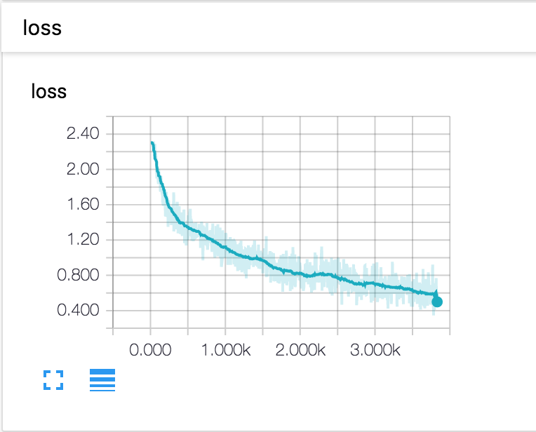
CNN Loss Curve
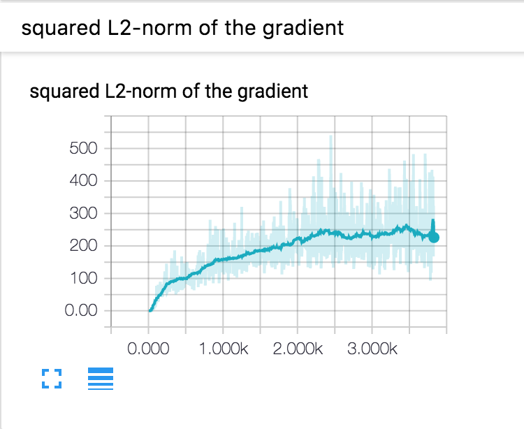
Curve of Squared L2-Norm
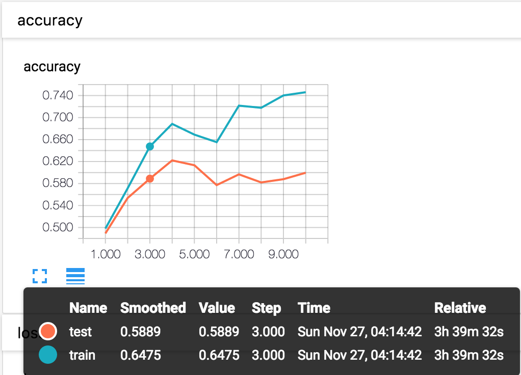
Training accuracy
Implementation Details of the Solver
Now we touch the details of the implementation of visualization in Solver. This will not show a complete implementation for the Solver class.
Step1: Generate SummaryWriters
If self.visualize == True, two SummaryWriters will be
generated by default, one for training and one for testing.
In [ ]:
class Solver(object):
    ...
    def __init__(self, model, train_dataiter, test_dataiter, **kwargs):
        ...
        self.visualize = kwargs.pop('visualize', False)

        if self.visualize:
            # Retrieve the summary directory. Create summary writers for training and test.
            self.summaries_dir = kwargs.pop('summaries_dir', '/private/tmp/newlog')
            self.train_writer = SummaryWriter(self.summaries_dir + '/train')
            self.test_writer = SummaryWriter(self.summaries_dir + '/test')
Step2: Set a Scalar Summary for Squared L2-norm of the Gradient
In [ ]:
def _step(self, batch, iteration):
    ...
    if self.visualize:
            Grad_norm = 0

        # Perform a parameter update
        for p, w in self.model.params.items():
            dw = grads[p]
            if self.visualize:
                norm = dw ** 2
                while not isinstance(norm, minpy.array.Number):
                    norm = sum(norm)
                Grad_norm += norm
            config = self.optim_configs[p]
            next_w, next_config = self.update_rule(w, dw, config)
            self.model.params[p] = next_w
            self.optim_configs[p] = next_config

        if self.visualize:
            grad_norm_summary = summaryOps.scalarSummary('squared L2-norm of the gradient', Grad_norm)
            self.train_writer.add_summary(grad_norm_summary, iteration)
    ...
Step3: Set a Scalar Summary for Training Loss
In [ ]:
def train(self):
        """
        Run optimization to train the model.
        """
        num_iterations = self.train_dataiter.getnumiterations(
        ) * self.num_epochs
        t = 0
        for epoch in range(self.num_epochs):
            start = time.time()
            self.epoch = epoch + 1
            for each_batch in self.train_dataiter:
                self._step(each_batch, t + 1)
                # Maybe print training loss
                if self.verbose and t % self.print_every == 0:
                    print('(Iteration %d / %d) loss: %f' %
                          (t + 1, num_iterations, self.loss_history[-1]))
                if self.visualize:
                    # Add scalar summaries of training loss.
                    loss_summary = summaryOps.scalarSummary('loss', self.loss_history[-1])
                    self.train_writer.add_summary(loss_summary, t + 1)

                t += 1
Step4: Set a Scalar Summary for Training/Validation Accuracy
In [ ]:
def train(self):
    ...
    for epoch in range(self.num_epochs):
        start = time.time()
        self.epoch = epoch + 1
        ...
        # evaluate after each epoch
        train_acc = self.check_accuracy(self.train_dataiter, num_samples=self.train_acc_num_samples)
        val_acc = self.check_accuracy(self.test_dataiter)
        self.train_acc_history.append(train_acc)
        self.val_acc_history.append(val_acc)
        ...
        if self.visualize:
            val_acc_summary = summaryOps.scalarSummary('accuracy', val_acc)
            self.test_writer.add_summary(val_acc_summary, self.epoch)
            train_acc_summary = summaryOps.scalarSummary('accuracy', train_acc)
            self.train_writer.add_summary(train_acc_summary, self.epoch)
        ...
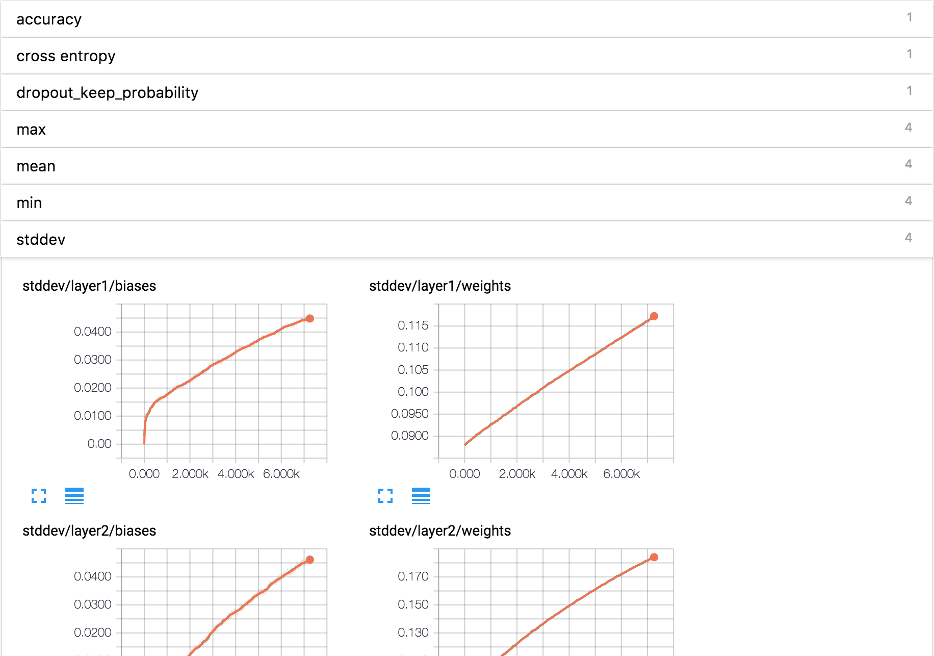
You could do whatever you want like cross entropy, dropout_keep_probability, mean, etc. This is a result from the TensorFlow’s tutorial on constructing a deep convolutional MNIST classifier: link.
MNIST Result