Visualization with TensorBoard

Visualization is a very intuitive way to inspect what is going on in a network. For that purpose, we integrate TensorBoard with MinPy. This tutorial begins with the Logistic Regression Tutorial, then moves on to a more advanced case with CNN.

Before trying this tutorial, make sure you have installed MinPy and TensorFlow.

Logistic regression

Set up as in the original tutorial.

from __future__ import absolute_import
from __future__ import division
from __future__ import print_function

import minpy.numpy as np
import minpy.numpy.random as random
from minpy.core import grad_and_loss
from examples.utils.data_utils import gaussian_cluster_generator as make_data
from minpy.context import set_context, gpu

Set up for Visualization. The related code is largely based on the source code from TensorFlow.

from minpy.visualization.writer import LegacySummaryWriter as SummaryWriter
import minpy.visualization.summaryOps as summaryOps

Declare the directory for log files which will be used for storing data during the training and later uploaded to TensorBoard later. The directory does not necessarily need to exist. The directory should start with /private where TensorBoard looks for log files by default.

summaries_dir = '/private/tmp/LR_log'

# Predict the class using multinomial logistic regression (softmax regression).
def predict(w, x):
    a = np.exp(np.dot(x, w))
    a_sum = np.sum(a, axis=1, keepdims=True)
    prob = a / a_sum
    return prob

def train_loss(w, x):
    prob = predict(w, x)
    loss = -np.sum(label * np.log(prob)) / num_samples
    return loss

"""Use Minpy's auto-grad to derive a gradient function off loss"""
grad_function = grad_and_loss(train_loss)

Create the writer for the trainning. You may replace /train with /test, /validation, etc. as you like.

train_writer = SummaryWriter(summaries_dir + '/train')

summaryOps.scalarSummary accepts a tag and a scalar as arguments and crates corresponding summary protos with scalars. train_writer then adds the summary proto to the log file. At the end of the training, close the writer.

The same trick works for all kinds of scalars. To clarify, it works for python scalars float, int, long, as well as one-element minpy.array.Array and numpy.ndarray.

Currently, Minpy only supports scalar summaries.

# Using gradient descent to fit the correct classes.
def train(w, x, loops):
    for i in range(loops):
        dw, loss = grad_function(w, x)
        # gradient descent
        w -= 0.1 * dw
        if i % 10 == 0:
            print('Iter {}, training loss {}'.format(i, loss))
        summary1 = summaryOps.scalarSummary('loss', loss)
        train_writer.add_summary(summary1, i)
    train_writer.close()

# Initialize training data.
num_samples = 10000
num_features = 500
num_classes = 5
data, label = make_data(num_samples, num_features, num_classes)

# Initialize training weight and train
weight = random.randn(num_features, num_classes)
train(weight, data, 100)

Iter 0, training loss [ 14.2357111]
Iter 10, training loss [ 1.60548949]
Iter 20, training loss [ 0.25217342]
Iter 30, training loss [ 0.10623146]
Iter 40, training loss [ 0.06312769]
Iter 50, training loss [ 0.0435785]
Iter 60, training loss [ 0.03269563]
Iter 70, training loss [ 0.02586649]
Iter 80, training loss [ 0.02122972]
Iter 90, training loss [ 0.01790031]

Open the terminal, and call the following command:

tensorboard --logdir=summaries_dir

Note you don’t need to include /private for the summaries_dir, so in this case the summaries_dir will be /tmp/LR_log.

Once you start TensorBoard, you should see the visualization of scalars in the EVENTS section as below. When you move your mouse along the curve, you should see the value at each step. You may change the size of the graph by clicking the button in the bottom-left corner.

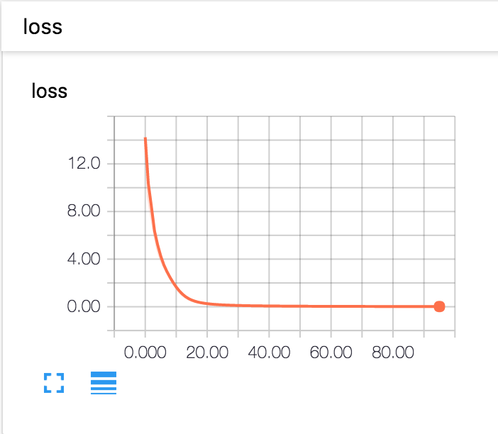
Loss History Interface

On the left hand side, you may decide to which extent you want to smooth the curve. You may choose one of the three choices as the horizontal axis of the graph. By checking Data download links, you may download the data in the format of .csv or .json. In the .csv or .json files, the data will be displayed in the form of [wall time - step - value].

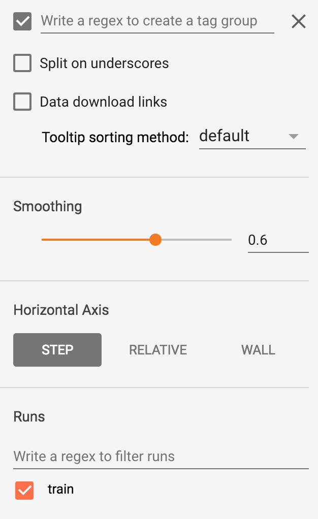
Control Interface