Autograd in MinPy
This tutorial is also available in step-by-step notebook version on github. Please try it out!
Writing backprop is often the most tedious and error prone part of a deep net implementation. In fact, the feature of autograd has wide applications and goes beyond the domain of deep learning. MinPy’s autograd applies to any NumPy code that is imperatively programmed. Moreover, it is seemlessly integrated with MXNet’s symbolic program (see for example). By using MXNet’s execution engine, all operations can be executed in GPU if available.
A Close Look at Autograd System
MinPy’s implementation of autograd is insprired from the Autograd
project. It computes a gradient
function for any single-output function. For example, we define a simple
function foo:
In [1]:
def foo(x):
    return x**2

foo(4)
Out[1]:
16
Now we want to get its derivative. To do so, simply import grad from
minpy.core.
In [2]:
import minpy.numpy as np  # currently need import this at the same time
from minpy.core import grad

d_foo = grad(foo)
In [3]:
d_foo(4)
Out[3]:
8.0
You can also differentiate as many times as you want:
In [4]:
d_2_foo = grad(d_foo)
d_3_foo = grad(d_2_foo)
Now import matplotlib to visualize the derivatives.
In [5]:
import matplotlib.pyplot as plt
%matplotlib inline
plt.rcParams['figure.figsize'] = (10.0, 8.0) # set default size of plots
plt.rcParams['image.interpolation'] = 'nearest'
plt.rcParams['image.cmap'] = 'gray'

x = np.linspace(-10, 10, 200)
# plt.plot only takes ndarray as input. Explicitly convert MinPy Array into ndarray.
plt.plot(x.asnumpy(), foo(x).asnumpy(),
         x.asnumpy(), d_foo(x).asnumpy(),
         x.asnumpy(), d_2_foo(x).asnumpy(),
         x.asnumpy(), d_3_foo(x).asnumpy())
plt.show()
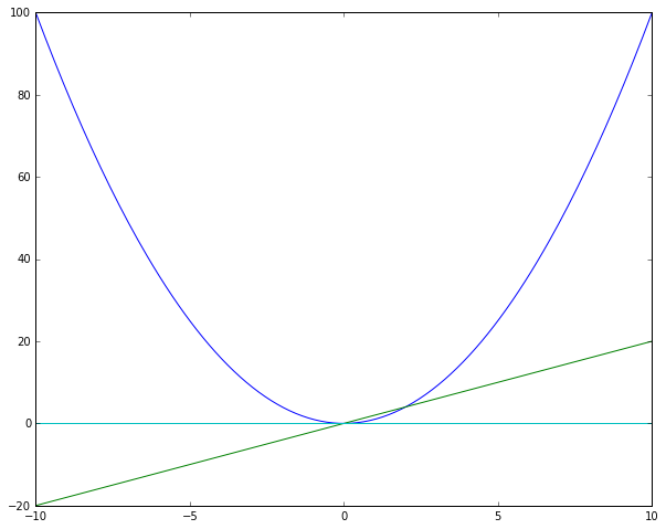
Just as you expected.
Autograd also differentiates vector inputs. For example:
In [6]:
x = np.array([1, 2, 3, 4])
d_foo(x)
Out[6]:
[ 2. 4. 6. 8.]
Gradient of Multivariate Functions
As for multivariate functions, you also need to specify arguments for
derivative calculation. Only the specified argument will be calcualted.
Just pass the position of the target argument (of a list of arguments)
in grad. For example:
In [7]:
def bar(a, b, c):
    return 3*a + b**2 - c
We get their gradients by specifying their argument position.
In [8]:
gradient = grad(bar, [0, 1, 2])
grad_array = gradient(2, 3, 4)
print grad_array
[3.0, 6.0, -1.0]
grad_array[0], grad_array[1], and grad_array[2] are
gradients of argument a, b, and c.
The following section will introduce a more comprehensive example on matrix calculus.
Autograd for Loss Function
Since in world of machine learning we optimize a scalar loss, Autograd is particular useful to obtain the gradient of input parameters for next updates. For example, we define an affine layer, relu layer, and a softmax loss. Before dive into this section, please see Logistic regression tutorial first for a simpler application of Autograd.
In [9]:
def affine(x, w, b):
    """
    Computes the forward pass for an affine (fully-connected) layer.
    The input x has shape (N, d_1, ..., d_k) and contains a minibatch of N
    examples, where each example x[i] has shape (d_1, ..., d_k). We will
    reshape each input into a vector of dimension D = d_1 * ... * d_k, and
    then transform it to an output vector of dimension M.
    Inputs:
    - x: A numpy array containing input data, of shape (N, d_1, ..., d_k)
    - w: A numpy array of weights, of shape (D, M)
    - b: A numpy array of biases, of shape (M,)
    Returns a tuple of:
    - out: output, of shape (N, M)
    """
    out = np.dot(x, w) + b
    return out

def relu(x):
    """
    Computes the forward pass for a layer of rectified linear units (ReLUs).
    Input:
    - x: Inputs, of any shape
    Returns a tuple of:
    - out: Output, of the same shape as x
    """
    out = np.maximum(0, x)
    return out

def softmax_loss(x, y):
    """
    Computes the loss for softmax classification.
    Inputs:
    - x: Input data, of shape (N, C) where x[i, j] is the score for the jth class
    for the ith input.
    - y: Vector of labels, of shape (N,) where y[i] is the label for x[i] and
    0 <= y[i] < C
    Returns a tuple of:
    - loss: Scalar giving the loss
    """
    N = x.shape[0]
    probs = np.exp(x - np.max(x, axis=1, keepdims=True))
    probs = probs / np.sum(probs, axis=1, keepdims=True)
    loss = -np.sum(np.log(probs) * y) / N
    return loss
Then we use these layers to define a single layer fully-connected network, with a softmax output.
In [10]:
class SimpleNet(object):
    def __init__(self, input_size=100, num_class=3):
        # Define model parameters.
        self.params = {}
        self.params['w'] = np.random.randn(input_size, num_class) * 0.01
        self.params['b'] = np.zeros((1, 1))  # don't use int(1) (int cannot track gradient info)

    def forward(self, X):
        # First affine layer (fully-connected layer).
        y1 = affine(X, self.params['w'], self.params['b'])
        # ReLU activation.
        y2 = relu(y1)
        return y2

    def loss(self, X, y):
        # Compute softmax loss between the output and the label.
        return softmax_loss(self.forward(X), y)
We define some hyperparameters.
In [11]:
batch_size = 100
input_size = 50
num_class = 3
Here is the net and data.
In [12]:
net = SimpleNet(input_size, num_class)
x = np.random.randn(batch_size, hidden_size)
idx = np.random.randint(0, 3, size=batch_size)
y = np.zeros((batch_size, num_class))
y[np.arange(batch_size), idx] = 1
Now get gradients.
In [13]:
gradient = grad(net.loss)
Then we can get gradient by simply call gradient(X, y).
In [14]:
d_x = gradient(x, y)
Ok, Ok, I know you are not interested in x’s gradient. I will show
you how to get the gradient of the parameters. First, you need to define
a function with the parameters as the arguments for Autograd to process.
Autograd can only track the gradients in the parameter list.
In [15]:
def loss_func(w, b, X, y):
    net.params['w'] = w
    net.params['b'] = b
    return net.loss(X, y)
Yes, you just need to provide an entry in the new function’s parameter
list for w and b and that’s it! Now let’s try to derive its
gradient.
In [16]:
# 0, 1 are the positions of w, b in the paramter list.
gradient = grad(loss_func, [0, 1])
Note that you need to specify a list for the parameters that you want their gradients.
Now we have
In [17]:
d_w, d_b = gradient(net.params['w'], net.params['b'], x, y)
With d_w and d_b in hand, training net is just a piece of
cake.
Less Calculation: Get Forward Pass and Backward Pass Simultaneously
Since gradient calculation in MinPy needs forward pass information, if
you need the forward result and the gradient calculation at the same
time, please use grad_and_loss to get them simultaneously. In fact,
grad is just a wrapper of grad_and_loss. For example, we can get
In [18]:
from minpy.core import grad_and_loss
forward_backward = grad_and_loss(bar, [0, 1, 2])
grad_array, result = forward_backward(2, 3, 4)
grad_array and result are result of gradient and forward pass
respectively.