RNN Tutorial
This tutorial describes how to implement recurrent neural network (RNN) on MinPy. RNN has different architecture, the backprop-through-time (BPTT) coupled with various gating mechanisms can make implementation challenging. MinPy focuses on imperative programming and simplifies reasoning logics. This tutorial explains how, with a simple toy data set and three RNNs (vanilla RNN, LSTM and GRU).
We do suggest you start with Complete solver and optimizer guide for MinPy’s conventional solver architecture.
Toy Dataset: the Adding Problem
The adding problem is a toy dataset for RNN used by many researchers. The input
data of the dataset consists of two rows. The first row contains random float
numbers between 0 and 1; the second row are all zeros, expect two randomly
chosen locations being marked as 1. The corresponding output label is a float
number summing up two numbers in the first row of the input data where marked as
1 in the second row. The length of the row T is the length of the input
sequence.
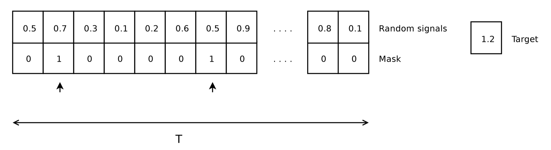
Figure: An example of the adding problem. 0.7 and 0.5 are chosen from the input data on the left and sum up as 1.2, the label on the right [1].
The paper [1] indicates that a less than 0.1767 Mean Square Error (MSE) proves the effectiveness of the network compared to the random guess. We set 0.1767 as the MSE baseline of our experiment.
We prepared an adding problem generator at examples.utils.data_utils.adding_problem_generator (
here). We append its
implementation as follows:
1 2 3 4 5 6 7 8 9 10 11 12 13 14 15 16 17 18 19 20 21 22 23 24 25 26 27 28 29 30 31 32 33 34 | def adding_problem_generator(N, seq_len=6, high=1):
""" A data generator for adding problem.
The data definition strictly follows Quoc V. Le, Navdeep Jaitly, Geoffrey E.
Hintan's paper, A Simple Way to Initialize Recurrent Networks of Rectified
Linear Units.
The single datum entry is a 2D vector with two rows with same length.
The first row is a list of random data; the second row is a list of binary
mask with all ones, except two positions sampled by uniform distribution.
The corresponding label entry is the sum of the masked data. For
example:
input label
----- -----
1 4 5 3 -----> 9 (4 + 5)
0 1 1 0
:param N: the number of the entries.
:param seq_len: the length of a single sequence.
:param p: the probability of 1 in generated mask
:param high: the random data is sampled from a [0, high] uniform distribution.
:return: (X, Y), X the data, Y the label.
"""
X_num = np.random.uniform(low=0, high=high, size=(N, seq_len, 1))
X_mask = np.zeros((N, seq_len, 1))
Y = np.ones((N, 1))
for i in xrange(N):
# Default uniform distribution on position sampling
positions = np.random.choice(seq_len, size=2, replace=False)
X_mask[i, positions] = 1
Y[i, 0] = np.sum(X_num[i, positions])
X = np.append(X_num, X_mask, axis=2)
return X, Y
|
Vanilla RNN
In Complete solver and optimizer guide, we introduced a simple model/solver architecture.
Implementing RNN in MinPy is very straightforward following the convention. The only
difference is the model part. The following MinPy code defines the vanilla RNN in
RNNNet class. We also include solver code for completeness. (You can find it in
this folder.)
1 2 3 4 5 6 7 8 9 10 11 12 13 14 15 16 17 18 19 20 21 22 23 24 25 26 27 28 29 30 31 32 33 34 35 36 37 38 39 40 41 42 43 44 45 46 47 48 49 50 51 52 53 54 55 56 57 58 59 60 61 62 63 64 65 66 | import minpy.numpy as np
from minpy.nn import layers
from minpy.nn.model import ModelBase
from minpy.nn.solver import Solver
from minpy.nn.io import NDArrayIter
from examples.utils.data_utils import adding_problem_generator as data_gen
class RNNNet(ModelBase):
def __init__(self,
batch_size=100,
input_size=2, # input dimension
hidden_size=64,
num_classes=1):
super(RNNNet, self).__init__()
self.add_param(name='Wx', shape=(input_size, hidden_size))\
.add_param(name='Wh', shape=(hidden_size, hidden_size))\
.add_param(name='b', shape=(hidden_size,))\
.add_param(name='Wa', shape=(hidden_size, num_classes))\
.add_param(name='ba', shape=(num_classes,))
def forward(self, X, mode):
seq_len = X.shape[1]
batch_size = X.shape[0]
hidden_size = self.params['Wh'].shape[0]
h = np.zeros((batch_size, hidden_size))
for t in xrange(seq_len):
h = layers.rnn_step(X[:, t, :], h, self.params['Wx'],
self.params['Wh'], self.params['b'])
y = layers.affine(h, self.params['Wa'], self.params['ba'])
return y
def loss(self, predict, y):
return layers.l2_loss(predict, y)
def main():
model = RNNNet()
x_train, y_train = data_gen(10000)
x_test, y_test = data_gen(1000)
train_dataiter = NDArrayIter(x_train,
y_train,
batch_size=100,
shuffle=True)
test_dataiter = NDArrayIter(x_test,
y_test,
batch_size=100,
shuffle=False)
solver = Solver(model,
train_dataiter,
test_dataiter,
num_epochs=10,
init_rule='xavier',
update_rule='adam',
task_type='regression',
verbose=True,
print_every=20)
solver.init()
solver.train()
if __name__ == '__main__':
main()
|
Layers are defined in minpy.nn.layers (here).
Note that data_gen is simply adding_problem_generator.
The key layer of vanilla RNN is also shown as follows:
1 2 3 4 5 6 7 8 9 10 11 12 13 14 15 16 17 18 19 20 | def rnn_step(x, prev_h, Wx, Wh, b):
"""
Run the forward pass for a single timestep of a vanilla RNN that uses a tanh
activation function.
The input data has dimension D, the hidden state has dimension H, and we use
a minibatch size of N.
Inputs:
- x: Input data for this timestep, of shape (N, D).
- prev_h: Hidden state from previous timestep, of shape (N, H)
- Wx: Weight matrix for input-to-hidden connections, of shape (D, H)
- Wh: Weight matrix for hidden-to-hidden connections, of shape (H, H)
- b: Biases of shape (H,)
Returns a tuple of:
- next_h: Next hidden state, of shape (N, H)
"""
next_h = np.tanh(x.dot(Wx) + prev_h.dot(Wh) + b)
return next_h
|
We see building rnn through imperative programming is both convenient and intuitive.
LSTM
LSTM was introduced by Hochreiter and Schmidhuber [2]. It adds more gates to control the process of forgetting and remembering. LSTM is also quite easy to implement in MinPy like vanilla RNN:
1 2 3 4 5 6 7 8 9 10 11 12 13 14 15 16 17 18 19 20 21 22 23 24 25 26 27 28 29 | class LSTMNet(ModelBase):
def __init__(self,
batch_size=100,
input_size=2, # input dimension
hidden_size=100,
num_classes=1):
super(LSTMNet, self).__init__()
self.add_param(name='Wx', shape=(input_size, 4*hidden_size))\
.add_param(name='Wh', shape=(hidden_size, 4*hidden_size))\
.add_param(name='b', shape=(4*hidden_size,))\
.add_param(name='Wa', shape=(hidden_size, num_classes))\
.add_param(name='ba', shape=(num_classes,))
def forward(self, X, mode):
seq_len = X.shape[1]
batch_size = X.shape[0]
hidden_size = self.params['Wh'].shape[0]
h = np.zeros((batch_size, hidden_size))
c = np.zeros((batch_size, hidden_size))
for t in xrange(seq_len):
h, c = layers.lstm_step(X[:, t, :], h, c,
self.params['Wx'],
self.params['Wh'],
self.params['b'])
y = layers.affine(h, self.params['Wa'], self.params['ba'])
return y
def loss(self, predict, y):
return layers.l2_loss(predict, y)
|
Layers are defined in minpy.nn.layers (here).
The key layer of LSTM is also shown as follows:
1 2 3 4 5 6 7 8 9 10 11 12 13 14 15 16 17 18 19 20 21 22 23 24 25 26 27 28 29 30 31 | def lstm_step(x, prev_h, prev_c, Wx, Wh, b):
"""
Forward pass for a single timestep of an LSTM.
The input data has dimension D, the hidden state has dimension H, and we use
a minibatch size of N.
Inputs:
- x: Input data, of shape (N, D)
- prev_h: Previous hidden state, of shape (N, H)
- prev_c: previous cell state, of shape (N, H)
- Wx: Input-to-hidden weights, of shape (D, 4H)
- Wh: Hidden-to-hidden weights, of shape (H, 4H)
- b: Biases, of shape (4H,)
Returns a tuple of:
- next_h: Next hidden state, of shape (N, H)
- next_c: Next cell state, of shape (N, H)
"""
N, H = prev_c.shape
# 1. activation vector
a = np.dot(x, Wx) + np.dot(prev_h, Wh) + b
# 2. gate fuctions
i = sigmoid(a[:, 0:H])
f = sigmoid(a[:, H:2*H])
o = sigmoid(a[:, 2*H:3*H])
g = np.tanh(a[:, 3*H:4*H])
# 3. next cell state
next_c = f * prev_c + i * g
next_h = o * np.tanh(next_c)
return next_h, next_c
|
The implementation of lstm_step is quite straightforward in MinPy.
GRU
GRU was proposed by Cho et al. [3]. It simplifies LSTM by using fewer gates and states. MinPy can also model GRU in an intuitive way:
1 2 3 4 5 6 7 8 9 10 11 12 13 14 15 16 17 18 19 20 21 22 23 24 25 26 27 28 29 30 31 | class GRUNet(ModelBase):
def __init__(self,
batch_size=100,
input_size=2, # input dimension
hidden_size=100,
num_classes=1):
super(GRUNet, self).__init__()
self.add_param(name='Wx', shape=(input_size, 2*hidden_size))\
.add_param(name='Wh', shape=(hidden_size, 2*hidden_size))\
.add_param(name='b', shape=(2*hidden_size,))\
.add_param(name='Wxh', shape=(input_size, hidden_size))\
.add_param(name='Whh', shape=(hidden_size, hidden_size))\
.add_param(name='bh', shape=(hidden_size,))\
.add_param(name='Wa', shape=(hidden_size, num_classes))\
.add_param(name='ba', shape=(num_classes,))
def forward(self, X, mode):
seq_len = X.shape[1]
batch_size = X.shape[0]
hidden_size = self.params['Wh'].shape[0]
h = np.zeros((batch_size, hidden_size))
for t in xrange(seq_len):
h = layers.gru_step(X[:, t, :], h, self.params['Wx'],
self.params['Wh'], self.params['b'],
self.params['Wxh'], self.params['Whh'],
self.params['bh'])
y = layers.affine(h, self.params['Wa'], self.params['ba'])
return y
def loss(self, predict, y):
return layers.l2_loss(predict, y)
|
Layers are defined in minpy.nn.layers (here).
The key layer of GRU is also shown as follows:
1 2 3 4 5 6 7 8 9 10 11 12 13 14 15 16 17 18 19 20 21 22 23 24 25 26 27 28 29 30 31 32 33 34 35 | def gru_step(x, prev_h, Wx, Wh, b, Wxh, Whh, bh):
"""
Forward pass for a single timestep of an GRU.
The input data has dimentsion D, the hidden state has dimension H, and we
use a minibatch size of N.
Parameters
----------
x : Input data, of shape (N, D)
prev_h : Previous hidden state, of shape (N, H)
prev_c : Previous hidden state, of shape (N, H)
Wx : Input-to-hidden weights for r and z gates, of shape (D, 2H)
Wh : Hidden-to-hidden weights for r and z gates, of shape (H, 2H)
b : Biases for r an z gates, of shape (2H,)
Wxh : Input-to-hidden weights for h', of shape (D, H)
Whh : Hidden-to-hidden weights for h', of shape (H, H)
bh : Biases, of shape (H,)
Returns
-------
next_h : Next hidden state, of shape (N, H)
Notes
-----
Implementation follows
http://jmlr.org/proceedings/papers/v37/jozefowicz15.pdf
"""
N, H = prev_h.shape
a = sigmoid(np.dot(x, Wx) + np.dot(prev_h, Wh) + b)
r = a[:, 0:H]
z = a[:, H:2 * H]
h_m = np.tanh(np.dot(x, Wxh) + np.dot(r * prev_h, Whh) + bh)
next_h = z * prev_h + (1 - z) * h_m
return next_h
|
gru_step stays close with lstm_step as expected.
Training Result
We trained recurrent networks shown early in this tutorial and use solver.loss_history to retrieve the MSE
history in the training process. The result is as follows.
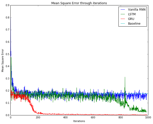
Figure: Result of training vanilla RNN, LSTM, GRU. A baseline of 0.1767 is also included.
rm e We observe that LSTM and GRU are more effective than vanilla RNN due to LSTM and GRU’s memory gates. In this particular case, GRU converges much faster than LSTM, probabuly due to fewer parameters.
Reference
| [1] | (1, 2) Q. V. Le, N. Jaitly, and G. E. Hinton, “A Simple Way to Initialize Recurrent Networks of Rectified Linear Units,” arXiv.org, vol. cs.NE. 04-Apr-2015. |
| [2] | S. Hochreiter and J. Schmidhuber, “Long Short-Term Memory,” Neural Computation, vol. 9, no. 8, pp. 1735–1780, Nov. 1997. |
| [3] | K. Cho, B. van Merrienboer, C. Gulcehre, D. Bahdanau, F. Bougares, H. Schwenk, and Y. Bengio, “Learning Phrase Representations using RNN Encoder-Decoder for Statistical Machine Translation,” arXiv.org, vol. cs.CL. 04-Jun-2014. |