Reinforcement learning with policy gradient

Deep Reinforcement Learning (RL) is another area where deep models are used. In this example, we implement an agent that learns to play Pong, trained using policy gradients. Since we are using MinPy, we avoid the need to manually derive gradient computations, and can easily train on a GPU.

The example is based on the problem and model described in Deep Reinforcement Learning: Pong from Pixels , which contains an introduction and background to the ideas discussed here.

The training setups in reinforcement learning often differ based on the approach used, making MinPy’s flexibility a great choice for prototyping RL models. Unlike the standard supervised setting, with the policy gradient approach the training data is generated during training by the environment and the actions that the agent chooses, and stochasticity is introduced in the model.

Specifically, we implement a PolicyNetwork that learns to map states (i.e. visual frames of the Pong game) to actions (i.e. ‘move up’ or ‘move down’). The network is trained using the RLPolicyGradientSolver.

See here for the full implementation.

PolicyNetwork

The forward pass of the network is separated into two steps:

1. Compute a probability distribution over actions, given a state.
2. Choose an action, given the distribution from (1).

These steps are implemented in the forward and choose_action functions, respectively:

class PolicyNetwork(ModelBase):
    def __init__(self,
                 preprocessor,
                 input_size=80*80,
                 hidden_size=200,
                 gamma=0.99):  # Reward discounting factor
        super(PolicyNetwork, self).__init__()
        self.preprocessor = preprocessor
        self.input_size = input_size
        self.hidden_size = hidden_size
        self.gamma = gamma
        self.add_param('w1', (hidden_size, input_size))
        self.add_param('w2', (1, hidden_size))

    def forward(self, X):
        """Forward pass to obtain the action probabilities for each observation in `X`."""
        a = np.dot(self.params['w1'], X.T)
        h = np.maximum(0, a)
        logits = np.dot(h.T, self.params['w2'].T)
        p = 1.0 / (1.0 + np.exp(-logits))
        return p

    def choose_action(self, p):
        """Return an action `a` and corresponding label `y` using the probability float `p`."""
        a = 2 if numpy.random.uniform() < p else 3
        y = 1 if a == 2 else 0
        return a, y

In the forward function, we see that the model used is a simple feed-forward network that takes in an observation X (a preprocessed image frame) and outputs the probability p of taking the ‘move up’ action.

The choose_action function then draws a random number and selects an action according to the probability from forward.

For the loss function, we use cross-entropy but multiply each observation’s loss by the associated discounted reward, which is the key step in forming the policy gradient:

    def loss(self, ps, ys, rs):
        step_losses = ys * np.log(ps) + (1.0 - ys) * np.log(1.0 - ps)
        return -np.sum(step_losses * rs)

Note that by merely defining the forward and loss functions in this way, MinPy will be able to automatically compute the proper gradients.

Lastly, we define the reward discounting approach in discount_rewards, and define the preprocessing of raw input frames in the PongPreprocessor class:

    def discount_rewards(self, rs):
        drs = np.zeros_like(rs).asnumpy()
        s = 0
        for t in reversed(xrange(0, len(rs))):
            # Reset the running sum at a game boundary.
            if rs[t] != 0:
                s = 0
            s = s * self.gamma + rs[t]
            drs[t] = s
        drs -= np.mean(drs)
        drs /= np.std(drs)
        return drs

class PongPreprocessor(object):
    ... initialization ...
    def preprocess(self, img):
        ... preprocess and flatten the input image...
        return diff

See here for the full implementation.

RLPolicyGradientSolver

The RLPolicyGradientSolver is a custom Solver that can train a model that has the functions discussed above. In short, its training approach is:

1. Using the current model, play an episode to generate observations, action labels, and rewards.
2. Perform a forward and backward pass using the observations, action labels, and rewards from (1).
3. Update the model using the gradients found in (2).

Under the covers, for step (1) the RLPolicyGradientSolver repeatedly calls the model’s forward and choose_action functions at each step, then uses forward and loss functions for step 2.

See here for the full implementation.

Training

Run pong_model.py to train the model. The average running reward is printed, and should generally increase over time. Here is a video showing the agent (on the right) playing after 18,000 episodes of training:

While this example uses a very simple feed-forward network, MinPy makes it easy to experiment with more complex architectures, alternative pre-processing, weight updates, or initializations!

Dependencies

Note that Open AI Gym is used for the environment.

Improved RL with Parallel Advantage Actor-Critic

The example above shows a basic model trained using the simplest policy gradient estimator, known as REINFORCE [1]. This gradient estimator is known to have high variance, resulting in slow training. Moreover, with the model and training process above we are limited to obtaining trajectories from a single environment at a time.

In this tutorial, we will address these issues by using an alternative gradient estimator with lower variance and introducing parallelism. In the end, we will be able to train a model to solve Pong in around an hour on a MacBook Pro [*]. All code can be found here.

We use ideas from the Asynchronous Actor-Critic (A3C) [2] algorithm. Broadly speaking A3C has two key features: asynchronous training that simultaneously uses trajectories from multiple environments, and the use of an estimated advantage function to reduce the variance of the policy gradient estimator.

Parallel training

A3C consists of a global model, with separate worker processes that have a local copy of the model. Each worker collects trajectories from its own environment, makes updates to the global model, then syncs its local model copy. Thus with n worker processes, updates are made using trajectories from n environments. Another feature of A3C is that updates are made every t_max (e.g. 20) steps instead of performing a single update per episode.

One insight is that we can achieve similar behavior as A3C without using multiple processes or copies of the model, when interacting with the environment is not expensive.

Instead, we can maintain n copies of the environment and at each step sequentially obtain n observations, then predict n different actions with the model using a single forward pass:

while not all_done:
    # Stack all the observations from the current time step.
    step_xs = np.vstack([o.ravel() for o in observations])

    # Get actions and values for all environments in a single forward pass.
    step_ps, step_vs = agent.forward(step_xs)
    step_as = agent.act(step_ps)

    # Step each environment whose episode has not completed.
    for i, env in enumerate(envs):
        if not done[i]:
            obs, r, done[i], _ = env.step(step_as[i])

            # Record the observation, action, value, and reward in the buffers.
            env_xs[i].append(step_xs[i])
            env_as[i].append(step_as[i])
            env_vs[i].append(step_vs[i])
            env_rs[i].append(r)

            # Store the observation to be used on the next iteration.
            observations[i] = preprocessors[i].preprocess(obs)

    ...

Then we can assemble the trajectories obtained from the n environments into a batch and update the model using a single backward pass:

# Perform update and clear buffers. Occurs after `t_max` steps
# or when all episodes are complete.
agent.train_step(env_xs, env_as, env_rs, env_vs)
env_xs, env_as = _2d_list(num_envs), _2d_list(num_envs)
env_rs, env_vs = _2d_list(num_envs), _2d_list(num_envs)

Thus the training is parallel in the sense that the trajectories are processed in the forward and backward passes for all environments in parallel. See train.py for the full implementation.

Since updates occur every t_max steps, the memory requirement for a forward and backward pass only increases marginally as we add additional environments, allowing many parallel environments. The number of environments is also not limited by the number of CPU cores.

One difference with A3C is that since the updates are not performed asynchronously, the most recent model parameters are always used to obtain trajectories from each environment. However, since the environments are independent the policy still explores different trajectories in each environment. Intuitively, this means that the overall set of samples used for training becomes more ‘diverse’ as we introduce more environments.

Improved gradient estimator

The ‘Advantage Actor-Critic’ in A3C refers to using an estimated advantage function to reduce the variance of the policy gradient estimator. In the REINFORCE policy gradient, the discounted return is used to decide which direction to update the parameters:

\[\nabla_{\theta} \log \pi_{\theta}(a_t|s_t)R_t\]

Where \(R_t\) is the total discounted return from time step \(t\) and \(\pi_{\theta}(a_t|s_t)\) is the probability of taking action \(a_t\) from state \(s_t\), given by the policy \(\pi_{\theta}\).

Alternatively, with an advantage function the direction of parameter updates is based on whether taking a certain action leads to higher expected return than average, as measured by the advantage function \(A(s_t,a_t)\):

\[\nabla_{\theta} \log \pi_{\theta}(a_t|s_t)A(s_t, a_t)\]

\[A(s_t, a_t) = Q(s_t,a_t) - V(s_t)\]

Where \(Q(s,a)\) is the action-value function that gives the expected return of taking action \(a_t\) from state \(s_t\), and \(V(s_t)\) is the state-value function, which gives the expected return from state \(s_t\).

Although the function \(Q(s,a)\) is unknown, we can approximate it using the discounted returns \(R\), resulting in an estimated advantage function:

\[\tilde{A}(s_t, a_t) = R_t - V(s_t)\]

An alternative estimator of the advantage function known as the Generalized Advantage Estimator (GAE) [3] has been developed by Schulman et al., which we implement here. The Generalized Advantage Estimator is as follows:

\[\tilde{A_t} = \sum_{l=0}^{\infty}(\gamma\lambda)^l\delta_{t+l}^V\]

\[\delta_{t}^V=r_t + \gamma V(s_{t+1}) - V(s_t)\]

Where \(r_t\) is the reward obtained at timestep \(t\), and \(V(s_t)\) is the state-value function, which we approximate in practice. \(\gamma\) and \(\lambda\) are fixed hyper-parameters in \((0,1)\).

To implement GAE, we therefore need to (a) implement the state-value function, (b) compute the advantages according to the equation above, and (c) modify the loss so that it uses the advantages and trains the state-value function.

(a) State-Value Function

We approximate the state-value function by modifying the policy network to produce an additional output, namely the value of the input state. Here, the state-value function is simply a linear transformation of the same features used to compute the policy logits:

def forward(self, X):
    a = np.dot(self.params['fc1'], X.T)
    h = np.maximum(0, a)

    # Compute the policy's distribution over actions.
    logits = np.dot(h.T, self.params['policy_fc_last'].T)
    ps = np.exp(logits - np.max(logits, axis=1, keepdims=True))
    ps /= np.sum(ps, axis=1, keepdims=True)

    # Compute the value estimates.
    vs = np.dot(h.T, self.params['vf_fc_last'].T) + self.params['vf_fc_last_bias']
    return ps, vs

(b) Compute Advantages

After assembling a batch of trajectories, we compute the discounted rewards used to train the value function, and the \(\delta\) terms and the advantage estimates for the trajectories from each environment.

for i in range(num_envs):
    # Compute discounted rewards with a 'bootstrapped' final value.
    rs_bootstrap = [] if env_rs[i] == [] else env_rs[i] + [env_vs[i][-1]]
    discounted_rewards.extend(self.discount(rs_bootstrap, gamma)[:-1])

    # Compute advantages for each environment using Generalized Advantage Estimation;
    # see eqn. (16) of [Schulman 2016].
    delta_t = env_rs[i] + gamma*env_vs[i][1:] - env_vs[i][:-1]
    advantages.extend(self.discount(delta_t, gamma*lambda_))

Notice the subtlety in the way we discount the rewards that are used to train the state-value function. If a trajectory ended mid-episode, we won’t know the actual future return of the trajectory’s last state. Therefore we ‘bootstrap’ the future return for the last state by using the value function’s last estimate.

(c) Loss Function

The loss function then uses the advantage estimates. A term is added to train the value function’s weights, using L2-loss with the observed discounted rewards as the ground truth. Finally, as noted in the A3C paper, an entropy term can be added that discourages the policy from collapsing to a single action for a given state, which improves exploration.

def loss(self, ps, actions_one_hot, vs, rs, advs):
    # Distribution over actions, prevent log of zero.
    ps = np.maximum(1.0e-5, np.minimum(1.0 - 1e-5, ps))

    # Policy gradient loss.
    policy_grad_loss = -np.sum(np.log(ps) * actions_one_hot * advs)

    # Value function loss.
    vf_loss = 0.5 * np.sum((vs - rs) ** 2)

    # Entropy regularizer.
    entropy = -np.sum(ps * np.log(ps))

    # Weight value function loss and entropy, and combine into the final loss.
    loss_ = policy_grad_loss + self.config.vf_wt * vf_loss - self.config.entropy_wt * entropy
    return loss_

See model.py for the full implementation.

Experiments

To see the effects of advantage estimation and parallel training, we train the model with 1, 2, 4, and 16 environments.

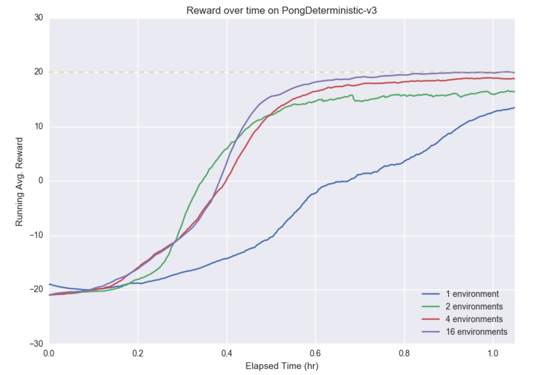
The plot shows the running average reward over time for various numbers of environments during the first hour of training. We can see that the improved gradient estimator allows all models to train quickly. Using 16 environments, the game is solved in around an hour.

We see that increasing the number of environments increases convergence speed in terms of wall-clock time; using 4 or 16 environments results in approaching the faster than using 2 environments or a single environment. This indicates that the increased number of samples per update outweighs the cost of processing the samples.

Moreover, training stability improves as more environments are used, as shown by the smooth, monotonic improvement with 16 environments versus the jagged, noisy improvement with 1 and 2 environments. One possible reason is that with more parallel environments, the samples used to update the policy are more diverse.

While a detailed analysis is outside the scope of this tutorial, we can see that the parallel Advantage Actor-Critic approach can train a model on the Pong environment in a fast and robust manner.

Note that we have kept the structure of the policy network the same as before; it is still a simple feed-forward network with 1 hidden layer.

Running

To train the model with default parameters, run:

python train.py

Here is a video showing the model after around an hour of training:

Feel free to experiment with other environments (which may require additional tuning), network architectures, or to use the code as a starting point for further research. For instance, we can also solve the CartPole environment:

python train.py --env-type CartPole-v0

[*]

Consistent with the Open AI A3C implementation [4], we use the PongDeterministic-V3 environment, which uses a frame-skip of 4. For this experiment, we define ‘solved’ as achieving a running average score of 20 out of 21 (computed using the previous 100 episodes). Note that for this version of Pong, humans were only able to achieve a score of -11 [5].

Reference

[1]	Williams, R.J. Simple statistical gradient-following algorithms for connectionist reinforcement learning. Machine Learning, 8(3):229–256, 1992.

[2]	Volodymyr Mnih, Adria Puigdomenech Badia, Mehdi Mirza, Alex Graves, Timothy P. Lillicrap, Tim Harley, David Silver, and Koray Kavukcuoglu. Asynchronous methods for deep reinforcement learning. In Proceedings of the 33rd International Conference on Machine Learning (ICML), pp. 1928–1937, 2016.

[3]	Schulman, John, Moritz, Philipp, Levine, Sergey, Jordan, Michael, and Abbeel, Pieter. High-dimensional continuous control using generalized advantage estimation. arXiv preprint arXiv:1506.02438, 2015b.

[4]	https://github.com/openai/universe-starter-agent#atari-pong. The A3C implementation in this repository was used as a reference when implementing the above.

[5]	https://openai.com/blog/universe/